Remarkably Stable GDP Growth – Part 3
First off, I want to thank Mark Sadowski for contributing, in a gadfly sort of way, to my thinking on this issue with his comments in Parts 1 and 2. So, this is not the part 3 post I had intended to write.
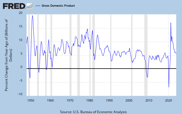
Mark suggested using a different transformation of the FRED NGDP series I’ve been looking at. Instead of taking YoY % change, he suggests using what FRED calls Compounded Annual Rate of Change [henceforth CARC.] Check the linked graphs and you’ll see there’s both more fine grain movement and swings to greater extremes in the CARC graph, and, as expected, the Standard Deviation values are higher. This is a different way of looking at the data. But is it a better way? I have no idea. If you have a convincing argument either way, let’s see it in comments.
Graph 1 shows the 13 Qtr Std Dev of CARC. It’s gross features are generally similar to the those of the graph of Std Dev of YoY Change. There’s the steep fall bottoming in 1964, the rise into a broad double peak in 1981-3, followed by a steep drop to a bottom in 1987. Then we see the humps caused by the ’91 and ’01 recessions, and finally the sharp rise and fall due to the Great Recession. [In the YoY graph some of these extremes are displaced by about a year.]

Graph 1 – 13 Qtr Std Dev of CARC
The major difference between the two graphs occurs after the 1987 bottom. While the YoY Std Dev graph continues to slope down, the CARC Std Dev graph moves in a generally horizontal direction between the two red lines drawn from the Q4 ’90 high of 2.95 and the Q3 ’12 low of 1.17. Note however, that if the ’91 recession had been worse or the ’01 recession milder, we would still perceive a downward tendency to the peaks.
The two most recent Std Dev readings are 1.27 and 1.22, so the precipitous fall following the great recession has ended. Note that similar lows occurred in Q3 ’98 and Q3 ’99 at 1.29 and 1.25, respectively and Q3 ’87 at 1.27. So – yes, we have recently observed the lowest Std Dev reading on record; but, no, it is not the lowest by any kind of great margin.
What accounts for the high Std Dev readings of the 70’s and 80’s – or, alternatively, what accounts for the low readings now? To explore this question, let’s indulge in a couple counter-factual exercizes. But first, let’s ponder what causes the Std Dev to be high, in general.
The main factors, in no particular order are
– The magnitude of the data values- frex, are they closer to 2 or to 22.
– The data spread envelope – frex, is it closer to +/- 10% or 110%.
– The data irregularity within the envelope – frex, does it gyrate wildly from extreme to extreme, or meander in a more leisurely fashion.
In the context of NGDP growth these factors become
– Average NGDP growth over a period of interest.
– The presence or absence of recessions.
– The growth variablilty in non-recessionary times.
Let’s explore the recession factor first. As it turns out, there are two features that come into play here: the depth of the recession, and the nature of the recovery. The deeper the recession, the greater the change in growth from the preceding period. The snappier the recovery, the greater the change in growth from the recessionary trough. Both of these things turn out to be important factors. Note in the FRED Graph of CARC that the recessions of the 70’s and 80’s had sharp, short rebounds in which NGDP growth was unusually high for one or more quarters. So both the recession and the recovery contributed to high Std Dev values. Now note the recoveries from the last three recessions. Very little snap back from ’91-92, only a little from ’01-02, and none at all from the Great Recession.
Here’s where our first counterfactual comes in. Suppose that the steep double dip recession of 1980-82 had never happened, or that it had occurred, but with only gradual recoveries from the troughs. These possibilities are illustrated in Graph 2.

Graph 2 – CARC with Counterfactuals
The blue line is actual CARC, The green line is a made-up version of CARC without the recessions. The pink line shows the recessions, but with smoothed recoveries and no snap back. Graph 3 shows the the 13 Qtr Std Devs for these data sets, with the same color coding.

Graph 3 – Std Dev of CARC with Counterfactuals
Simply eliminating the snap back recoveries brings the Std Dev down by 2 to 2.5 points. Eliminating the recessions entirely brings the Std Dev down from just over 6.5 to just over 2.5, a reduction of almost 60%.
Note also the sharp jump in Std Dev at Q2 ’78, and the following plateau. This is entirely due to a single quarter of ridiculously high NGDP growth during the moribund Carter administration, and illustrates how a single anomalous data point can distort the Std Dev calculation for an extended period. The plateau ends at Q3 ’81 when this point falls out of the 13 Q data kernel.
In comments to Part 1, Mark Sadowski asked if lower volatility isn’t a good thing. My answer is — only maybe. If it’s caused by avoiding recessions, then yes. But if it’s caused by lopping off the potential tops of recoveries, such as what we have experience these last three years, then no – not at all.
Here’s another counterfactual to ponder. What would the Std Dev of CARC have been in the period we just looked at if NGDP growth were at the current level, but the relative volatility had remained the same? From Q2 ’78 through Q3 ’84, CARC averaged 9.93%. Suppose a counterfactual of 4.01% average CARC, which is what we have experience from Q3 ’09 through Q1 ’13, the recovery from the great recession. This is illustrated in Graph 4.

Graph 4 – Early 80’s Counterfactual
The dark blue line is the actual CARC data. The horizontal blue line is the period average of 9.93. The brown line is the counterfactual CARC data, constructed by having each point be above or below the average of 4.01 [brown horizontal line] by the same percentage as the corresponding real data point. The light blue and red lines show the 13 Q Std Dev values for the two data sets, respectively. The Std Dev value for the entire real data set is 5.92. The Std Dev for the counterfactual data set is 2.39. This is again a reduction of just about 60%.
So, if you take the early 80’s data and eliminate the recessions, Std Dev for the flatish period from Q3 ’81 to Q1 ’84 drops by 58% from 6.34 to 2.65.
Also, if you consider the volatility level of Q2 ’78 to Q4 ’84 along with the CARC level following the Great Recession, the Std Dev drops by 59.7% from 5.92 to 2.39. So this gives me another answer to Mark’s question: If the low Std Dev is an artifact of low NGDP growth, then no, it’s not a good thing at all.
These examples suggest that both the occurrence of recessions and the high level of NGDP growth just before the start of the alleged great moderation were about equally as important in contributing to the high Std Dev of that era.
So I have to modify my idea about the relative importance of these two factors in making Std Dev high or low. A low NGDP growth rate is only AS important, not MORE important than avoiding recessions
Remember, the point of this exercise is to show that the low volatility of current NGDP growth is neither remarkable, nor necessarily a particularly good thing. I think I’m getting there.
Next, In Part 4, I’ll look at what I originally intended to look at in Part 3. Stay tuned.
“First off, I want to thank Mark Sadowski for contributing, in a gadfly sort of way, to my thinking on this issue with his comments in Parts 1 and 2.”
Anything to upset the apple cart, er, status quo.
“The two most recent Std Dev readings are 1.27 and 1.22, so the precipitous fall following the great recession has ended. Note that similar lows occurred in Q3 ’98 and Q3 ’99 at 1.29 and 1.25, respectively and Q3 ’87 at 1.27. So – yes, we have recently observed the lowest Std Dev reading on record; but, no, it is not the lowest by any kind of great margin.”
This depends on the length of periods considered. There’s nothing written in stone saying one has to look at periods of 13 quarters in length. (In fact, 13 quarters is an exceptionally odd choice.) If one chooses something slightly more conventional say such as 12 quarters or three years then the the two lowest standard deviations on record are the 12 quarter periods ending in 2012Q3 (1.02) and 2012Q2 (1.08) and the next one is 1999Q3 (1.26) which is more than just slightly higher.
In any case I think you’re getting a little pedantic here. Lowest ever volatility is still lowest ever.
“In comments to Part 1, Mark Sadowski asked if lower volatility isn’t a good thing. My answer is — only maybe. If it’s caused by avoiding recessions, then yes. But if it’s caused by lopping off the potential tops of recoveries, such as what we have experience these last three years, then no – not at all.”
But if you don’t have a recession in the first place then there’s nothing to recover from, is there? The problem is that the Fed is behaving as though NGDP did not fall 14% or so below trend. The current trajectory might have been OK otherwise.
Under NGDP level targeting (NGDPLT) you target the *level* of NGDP with the level growing at a constant rate. If it falls significantly below that level you will almost certainly experience a recession. If this occurs the thing to do is to return NGDP back to the target level (not to behave as though nothing had ever happened).
Now as to what the appropriate NGDP level, and rate of change in the level, that is a matter of opinion.
Mark –
I’ll admit to being perhaps even inordinately fond of the number 13, But, if you’ll check the block quote at the beginning of Part 1 of this series, you find that you picked it, and then I went with it.
And here in part 3, I’ve gone with CARC, which you also picked. I’m willing to indulge in this kind of accommodation, in hopes of avoiding the sort of, “Oh, but what about this” nonsense that have historically plagued Mike Kimel’s posts. So its really not obvious to me that I should tolerate much more goal post migration.
Truth is, twelve quarters vs 13 is a pretty trivial change, and it results in some very minor – and very brief – number alterations, as you point out. But the fact is, you’re cherry picking. With a 12 Q kernel, the St Dev value falls sooner, and just a bit farther because you’re removing an extreme CARC value from a one-unit-smaller smaller data set. The same thing happened in ’74, ’77, ’78, ’94, and ’03, the latter being quite an extreme example. In every one of those instances, the 12 Q Std Dev soon moved back above the 13 Q, as is happening now. This data artifact rates a MEH!
The 12 Q and 13 Q Std Dev values twine around each other over time, so I would make nothing at all of a slight difference after an extreme event. If you think a transient difference between 1.02 and 1.17 or 1.26 is significant when the curve has just dropped from values over 4, then I think you’re really stretching to make your point.
Meanwhile, you chose to ignore that the current low level of CARC is a major driver for low St Dev values.
Is it pedantic to try to understand what drives a phenomenon that has seemed very important over the last coupe of decades? Or is it that this understanding does not comport well with your view of the world?
Really, calling pedantic on me is an exceptionally odd criticism, and not well warranted.
http://www.thefreedictionary.com/pedantic
The FED has kept interest rates historically low for an extended period while engaging in unprecedented open market activities. It’s fine to talk about NGDP targeting, but what are they supposed to do to achieve some target level?
Cheers!
JzB
As you said in part 2:
“I like 13 because it’s a Fibonacci number, but it’s also the duration in quarters of the current remarkably stable GDP growth, so let’s see how it works over time.”
I never ever suggested that looking at periods of length 13 quarters was either the ideal or only way to go about a systematic analysis of NGDP volatility. That is purely your personal fixation not mine.
I personally don’t think it really matters much how long the periods are. However if you look at periods of three years in length, somethign which is far more conventional, there are 253 such periods. Of the seven periods of this length with the lowest standard deviation four of them are the periods ending in 2012Q2, 2012Q3, 2012Q4 and 2013Q1, in other words the four consecutive quarters including the most recent one.
“Meanwhile, you chose to ignore that the current low level of CARC is a major driver for low St Dev values.”
I ignore it because it is largely irrelevant. There is no coherent mechanism by which the rate of growth of NGDP is the primary determinent the volatility of NGDP growth.
“The FED has kept interest rates historically low for an extended period while engaging in unprecedented open market activities. It’s fine to talk about NGDP targeting, but what are they supposed to do to achieve some target level?”
Absolute nonsense. The Federal funds rate has only been at its current level for just over four and a half years. The previous time short term interest rates were near zero was from 1932 to 1947 a period of 15 years.
[That new post comment button is very hard to see. I wasn’t quite finished.]
As for “open market operations”, it wasn’t only open market operations that led to this (it was also unsterilized gold inflows), but in the 1940s the monetary base was even larger that it is today relative to GDP, so this is not without precedent.
If NGDP volatility can be kept at unprecedently low levels despite being subject to repeated fiscal policy and other negative aggregate demand shocks, as it has over the past three years, then obviously monetary policy is not having any difficulty at all setting the level of aggregate demand which for all intents and purposes is NGDP.
“Meanwhile, you chose to ignore that the current low level of CARC is a major driver for low St Dev values.”
I ignore it because it is largely irrelevant. There is no coherent mechanism by which the rate of growth of NGDP is the primary determinent the volatility of NGDP growth.
You ignore it because you don’t like it. That is conformation bias in action. Small data value magnitudes give small Std Dev values. I demonstrated that in the post, and really, it’s blazingly obvious. If you refuse to acknowledge it, then fine, your Weltanschauung is secure. Thank you for playing, and have a nice day.
Cheers!
JzB
Absolute nonsense. The Federal funds rate has only been at its current level for just over four and a half years. The previous time short term interest rates were near zero was from 1932 to 1947 a period of 15 years.
Only 4 1/2 years. Wow. Really – wow.
As far back as FRED data goes – 1954 – there has been no period when the Fed Funds rate was even close to steady at ANY level for 4 1/2 years, and no time at which the current low level has been approached for as much as a single day.
But this wasn’t true from during the great depression through the near aftermath of WW II. Point taken.
You are quite profligate with your use of the word “nonsense.” I believe the translation into Standard American is “something Mark disagrees with.”
Cheers!
JzB
“Small data value magnitudes give small Std Dev values.”
In a normal distribution the mean and standard deviation are *independent* of each other. That is, one could be large or small and the other large or small without any influence on each other.
It is true they *may* be linked so that larger, means tend to have larger standard deviations. However there is no theoretical reason why the the mean and standard deviation of NGDP growth rates should be dependent on each other.
“I demonstrated that in the post, and really, it’s blazingly obvious.”
The average rate of growth of U.S. NGDP happens to be positively correlated with the standard deviation of U.S. NGDP growth rates over the Great Disinflation which just happens to overlap with the Great Moderation when NGDP volatility declined.
In three year periods ending in 1954 to 1978, which overlaps with the Great Inflation, the 12 quarter standard deviations of the compounded annual rate of change in NGDP are significantly *negatively* correlated with the average rate of change in NGDP. In other words NGDP became *less volatile* as its average rate of change *increased*.
Looking internationally, FRED has NGDP for the eurozone from 1995 and for Japan from 1994. The 12 quarter average rates of growth in NGDP and the standard deviations of the compounded annual rates of NGDP growth are significantly *negatively* correlated in both cases.
If you look at the period before the existence of the Fed (e.g. see Measuringworth) you will find that the ten year standard deviations of NGDP growth are significantly *negatively* correlated with the average rate of change in NGDP growth in ten year periods ending from 1816 to 1902.
There are many other counterexamples.
Oops. I meant 1816 to *1857*.
I could explain where the *1902* came from but it’s a long story. It comes from trying to do to many things at the same time.
“In three year periods ending in 1954 to 1978…”
should read
“In three year periods ending in 1957 to 1978…”